Tutorial

Background

In this tutorial, we seek to measure the temperature of an exoplanet atmosphere via transmission spectroscopy. As a transiting planet passes in front of its host star, the planet will appear largest at wavelengths where the planet’s atmosphere is opaque. For this toy model, we will include water opacity as the only absorbing species in the atmosphere.

As in Fisher & Heng (2018), we compute the apparent radius of the exoplanet as a function of wavelength given by

\[R = R_0 + H (\gamma + \ln \tau)\]

where \(R_0\) is the fiducial radius of the exoplanet, \(H\) is the atmospheric scale height, \(\gamma\) is the Euler-Mascheroni constant, and \(\tau\) is

\[\tau = \frac{\kappa_\lambda P_0}{g} \sqrt{\frac{2\pi R_0}{H}}\]

where \(\kappa_\lambda\) is the wavelength-dependent opacity, \(P_0\) is the reference pressure probed by transmission spectroscopy, and \(g\) is the surface gravity. The pressure scale height \(H\) is

\[H = \frac{k_B T}{\mu g}\]

where \(k_B\) is Boltzmann’s constant, \(T\) is the temperature, and \(\mu\) is the mean molecular weight.

We have generated an example transmission spectrum with random normal noise with \(T = 1500\) K, and in the following examples we will attempt to “retrieve” that temperature directly from the spectrum. First we’ll solve for the approximate temperature (without uncertainties) using \(\chi^2\) minimization. Then we’ll solve for the temperature and its uncertainty assuming Gaussian uncertainties using a likelihood function and Markov Chain Monte Carlo (MCMC). Finally, we’ll use approximate Bayesian computation (ABC) without defining a proper likelihood.

\(\chi^2\) minimization

First we will access the pre-generated example spectrum contained within the retrieval module, like so:

from retrieval import Planet, get_example_spectrum

import numpy as np
from scipy.optimize import fmin_l_bfgs_b
import astropy.units as u

example_spectrum = get_example_spectrum()

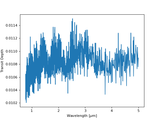
plt.plot(example_spectrum[:, 0], example_spectrum[:, 1])
plt.xlabel('Wavelength [$\mu$m]')
plt.ylabel('Transit Depth')
plt.show()

(Source code, png, hires.png, pdf)

The transit depth spectrum spans the near-infrared, where water opacity is significant, giving rise to the J, H and K bands visible in this transmission spectrum near 1.2, 1.6, and 2.2 microns, for example.

Now we create an instance of the Planet object, which requires us to specify the planet’s mass, radius, atmospheric pressure and mean molecular weight:

planet = Planet(1 * u.M_jup, 1 * u.R_jup, 1e-3 * u.bar, 2.2 * u.u)

With the exoplanet’s properties defined, we can now solve for the temperature in the atmosphere, using the forward model described in the equations above. We’ll define the \(\chi^2\) by comparing the example transmission spectrum with instances of the forward model at different temperatures, varying the temperature until we find good agreement between the model and observations:

def chi2(p):
    """
    Compute the chi^2 for the model with parameters `p`
    """
    temperature = p[0] * u.K
    return np.sum((example_spectrum[:, 1] -
                   planet.transit_depth(temperature).flux)**2 /
                  example_spectrum[:, 2]**2)

initp = [1700]  # K

bestp = fmin_l_bfgs_b(chi2, initp, approx_grad=True,
                      bounds=[[500, 5000]])[0][0]

The resulting best-fit temperature is:

>>> print(bestp)  
1509.4660124465638

which is close to the temperature used to generate the example spectrum, so we have demonstrated that the forward model is producing a sufficient approximation to the observed spectrum. It was straightforward in this example above to fit for the temperature, but it will take a bit more effort to find the uncertainty on the temperature.

MCMC with a likelihood

One computationally expensive but easy-to-implement technique for measuring the uncertainty on the fitting parameter is Markov Chain Monte Carlo (MCMC). MCMC is a Bayesian technique, and uses some of the concepts straight out of Bayes’ theorem,

\[P\left( \theta \vert D \right) = \frac{ \pi\left( \theta \right) ~{\cal L}\left( D \vert \theta \right) }{ {\cal Z} \left( D \right)}.\]

The prior distribution, denoted by \(\pi(\theta)\), represents your prior beliefs about the fitting parameters \(\theta\).

The likelihood function, \({\cal L}( D \vert \theta)\), is the relationship between the data (\(D\)), model and measurement noise. The goal of MCMC is to numerically evaluate the numerator in the equation on the right hand side of the equation to solve for the posterior distribution \(P\left( \theta \vert D \right)\).

To do so, we must first describe the prior and likelihood, respectively:

from emcee import EnsembleSampler

def lnprior(theta):
    """
    Log-prior
    """
    temperature = theta[0]

    if 500 < temperature < 5000:
        return 0
    return -np.inf

def lnlikelihood(theta):
    """
    Log-likelihood
    """
    temperature = theta[0] * u.K
    model = planet.transit_depth(temperature).flux
    lp = lnprior(theta)
    return lp + -0.5 * np.sum((example_spectrum[:, 1] - model)**2 /
                               example_spectrum[:, 2]**2)

We’ve chosen a flat log-prior that expects the temperature to sit between 500 and 5000 K, which might represent our sensible rough estimates for the minimum and maximum temperature a planet might have given its orbital distance and host star’s spectral type. The log-likelihood we have chosen for this example is the sum of the log-prior and \(-0.5 \chi^2\). This is a natural choice for the likelihood given Gaussian, uncorrelated uncertainties for the transit depth measurements.

We can now sample the posterior distribution with MCMC using emcee like so:

nwalkers = 4
ndim = 1

p0 = [[1500 + 10 * np.random.randn()]
      for i in range(nwalkers)]

with Pool() as pool:
    sampler = EnsembleSampler(nwalkers, ndim, lnlikelihood, pool=pool)
    sampler.run_mcmc(p0, 1000)

plt.hist(sampler.flatchain)
plt.xlabel('Temperature [K]')
plt.show()

(Source code, png, hires.png, pdf)

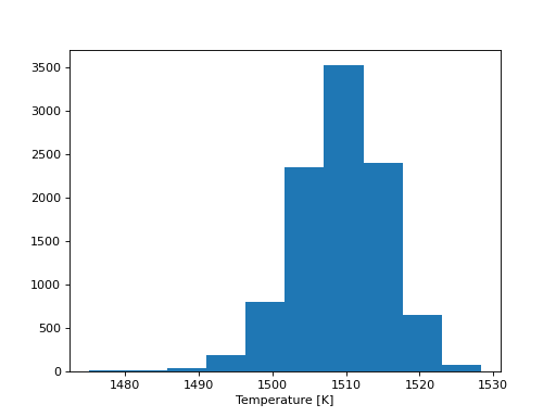
The algorithm produces a “chain” of posterior samples for the temperature of the atmosphere, which we see is roughly Gaussian in shape, yielding a temperature measurement of \(T \approx 1510 \pm 10\) K.

ABC without a likelihood

There can be situations where the likelihood is expensive or difficult to compute. In these situations, it can be useful to use approximate Bayesian computation, a technique for estimating posterior distributions without computing a likelihood.

Let’s imagine for a moment that the spectrum we’re trying to retrieve has been observed at very high resolution, with millions or billions of spectral channels, making the \(\chi^2\) expensive to compute. In this case, it is computationally more efficient to compute a summary statistic which reduces the dimensionality of the problem.

We can use domain knowledge to construct a summary statistic that has some physically sensible meaning. In this tutorial we will use the difference in transit depth on and off of a water absorption band as a summary statistic for the ABC technique. In this tutorial, the only free parameter is the temperature, so varying the temperature will vary the scale height of the atmosphere, which drives changes in the absorption band depth.

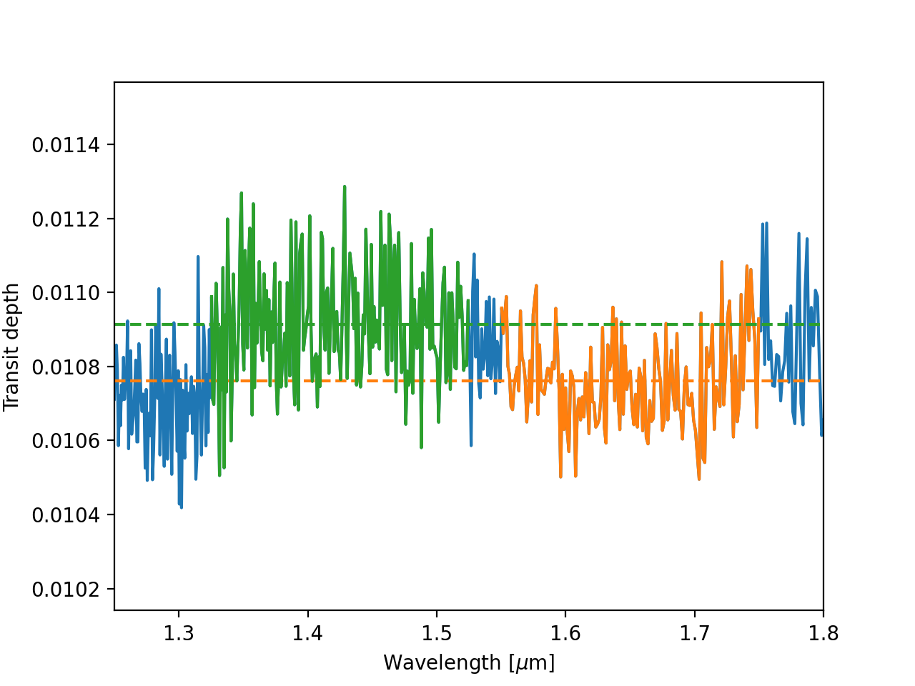
Below, let’s plot water’s near-infrared transparency feature which we usually call the H band (orange), and the water absorption band at just-shorter wavelengths than the H band (green), and the rest of the spectrum (blue).

on_h_band = np.abs(wavelength - 1.65) < 0.1
off_h_band = np.abs(wavelength - 1.425) < 0.1

depth_on = transit_depth[on_h_band].mean()
depth_off = transit_depth[off_h_band].mean()
depth_difference_observed = (depth_off - depth_on) / depth_off

(Source code, png, hires.png, pdf)

The “band depth,” or mean difference in transit depth on and off of this water absorption feature, is proportional to the temperature of the atmosphere in this toy model. We can therefore define a “distance” between the observed spectrum and simulated (forward) models of the spectrum which is simply the absolute difference between the band depth in the simulated spectrum and the band depth in the observed spectrum.

def distance(theta):
    temperature = theta[0] * u.K
    model = planet.transit_depth(temperature).flux
    depth_difference_simulated = abs((model[off_h_band].mean() -
                                      model[on_h_band].mean()) /
                                     model[off_h_band].mean())
    return abs(depth_difference_simulated - depth_difference_observed)

This is a dimensionality reduction step because we’re reducing the entire spectrum to a single number. One must take care to choose a summary statistic which unambiguously varies with the fitting parameters of interest – in general it is not possible to prove that your choice of summary statistic is “sufficient”.

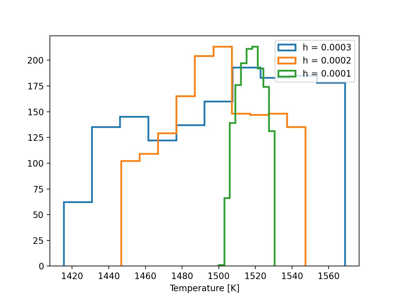
Next we construct a simple rejection sampling algorithm, which varies the temperature by a small amount, and tests the difference in band depth between the simulated and observed spectra. If the difference is within some tolerance specified by the user, the step is accepted into a chain, or otherwise it is discarded. We repeat this procedure for three different tolerances to demonstrate how the variance of the posterior decreases as the tolerance decreases:

init_temp = 1500
n_steps = 1500

thresholds = [3e-4, 2e-4, 1e-4]

for threshold in thresholds:
    # Create chains for the distance and temperature
    distance_chain = [distance([init_temp])]
    temperature_chain = [init_temp]

    # Set some indices
    i = 0
    total_steps = 1

    # Until the chain is the correct number of steps...
    while len(temperature_chain) < n_steps:
        # Generate a trial temperature
        total_steps += 1
        trial_temp = temperature_chain[i] + 10 * np.random.randn()

        # Measure the distance between the trial step and observations
        trial_dist = distance([trial_temp])

        # If trial step has distance less than some threshold...
        if trial_dist < threshold:
            # Accept the step, add values to the chain
            i += 1
            temperature_chain.append(trial_temp)
            distance_chain.append(trial_dist)

    # Compute the acceptance rate:
    acceptance_rate = i / total_steps
    print(f"h = {threshold}, acceptance rate = {acceptance_rate}")

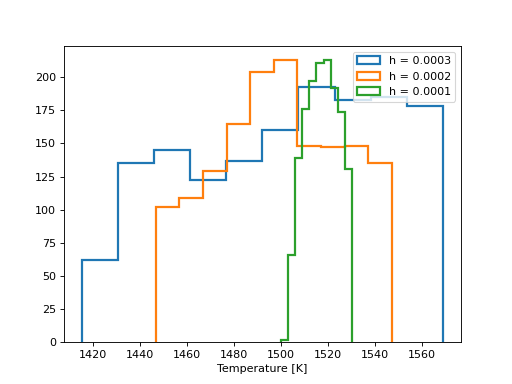
    plt.hist(temperature_chain, histtype='step', lw=2,
             label=f'h = {threshold}')
plt.legend()
plt.xlabel('Temperature [K]')
plt.show()

(Source code, png, hires.png, pdf)

In the above approximate posterior distributions, the variance of the posterior decreases as the tolerance \(h\) decreases. The parameter \(h\) represents the trade off between precision in the posterior approximation and computation time. The posterior distribution approximations should converge towards the “true” posterior distribution which you might recover with non-approximate Bayesian inference techniques like MCMC.

Taking the most computationally expensive and most accurate posterior approximation above (green), we estimate the temperature \(T \approx 1515 \pm 15\) K, roughly consistent with the expectation from MCMC above.